Test and Measurements Using Electrical Engineering Lab Equipment
Equipment
The equipment you will encounter in Electrical Engineering Laboratories are specially designed to provide power to your circuit, apply stimulus to your circuit, and measure your circuit’s response, while not changing or adding parasitic affects to your circuit.
Knowing and using the correct terminology of the equipment is important.
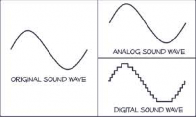
The circuits you will encounter in this class are known as “analog circuits” as opposed to “digital” or “mixed signal” circuits. The world around us is analog—we hear sounds as continuous waves. A computer, on the other hand, operates in the digital domain and only understands discrete values. So, we use analog circuits to sense the world around us and digital circuits to perform computations. To interface these two worlds one may build a mixed-signal circuit.
Test and Measurement Instrumentation is broken into three parts:
- Power
- Input or Stimulus
- Output or Measurement
Power
Power is applied to a circuit by use of a power supply, which the circuit needs to work. You can think of a power supply as the energy that the circuit uses to do work. Input stimulus supplies power to the input of your circuit, but only to the input. The output measurement instruments do not supply power to the circuit. In fact input stimulus and output measurement instruments are non-invasive, and won’t affect the circuit’s operation, allowing for accurate measurements of the circuit without affecting the circuit’s performance.
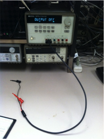
Figure 1
The power supply on the bench has three DC power supplies in one case: +6, +25, and -25 Volts DC. Connecting the power supply to the circuit may be accomplished in many ways.
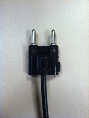
Figure 2
One way to couple the power supply to your circuit is by using a cable having a plug similar to Figure 2. This cable is plugged into the power supply’s (+) and (-) terminals. The tab that can be seen on the right side of the plug, plugs into the negative, or ground, or return of the power supply as shown in Figure 3.
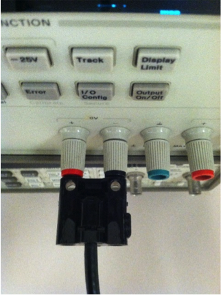
Figure 3
Ground for a power supply is signified by a black terminal, or the (-) label. Earth ground is signified by a green terminal, which should not be used for any labs. Earth ground is a return for all machinery and appliances and tends to be quite noisy, which is bad for experiments and for making measurements on circuits. Sometimes ground terminals can be red and labeled with (-), which in this case the red terminal is called “return,” and acts like a ground for your circuit.
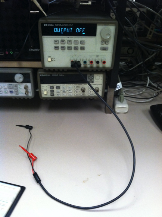
Figure 4
Figure 4 shows the cable coupled to the +6 Volts DC (VDC) power supply. The ends of the cable are clips, which are commonly referred to as “cue balls.” The plugs that insert into the power supply are commonly referred to as “banana plugs,” because they are in the shape of a banana.
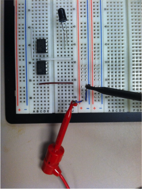
Figure 5
Figure 5 shows the cue balls coupled to a circuit being built on a prototyping board commonly referred to as a “breadboard.” The breadboard is designed to allow for easy and quick prototyping of electronic circuits, by allowing wires (having a solid core) and legs of electronic components, to be inserted into the holes making electronic connections. The electronic connections of a breadboard are laid out in vertical columns and horizontal rows (as the breadboard is orientated in Figure 5). The vertical holes, identified by red and blue stripes, as seen in Figure 5, are all shorted together (a term meaning that they are all connected) and run the entire length of the breadboard. These are typically used for power supplies. In Figure 5 you can see the black cue ball, which is coupled to the power supply’s ground or (-) (not seen in Figure 5), is clipped to a wire, which is inserted into the (-) blue vertical row of holes. All of the holes running vertically along the blue line are now access points to the power supply ground for your circuit. Likewise, the red cue ball, which is coupled the (+) side of the power supply (not seen in Figure 5) is clipped to a wire, which is inserted in the (+) red column of the breadboard. The red (+) column, like the blue (-) column, runs the whole length of the breadboard and serves as power supply (+) access points for your circuit.
All other holes in the breadboard are shorted horizontally, and are separated by a trough or indentation that runs vertically as illustrated in Figure 5. Also, note that in Figure 5, there are two breadboards mounted side-by-side, which are not connected. Having two breadboards mounted side-by-side accommodates larger circuits. A single breadboard is usually sufficient for most circuit developments. We are using the left breadboard. In Figure 5, there is a brown wire, which has been inserted into the breadboard, which couples two horizontal rows. Without the brown wire, the two adjacent horizontal rows would be separated. In Figure 5, the integrated circuits (IC’s) are placed incorrectly. The correct way to place the IC’s is so that they straddle the trough, which will isolate the two sides of the IC. In Figure 5, the legs on opposite sides of the IC’s will be shorted, and will not function.
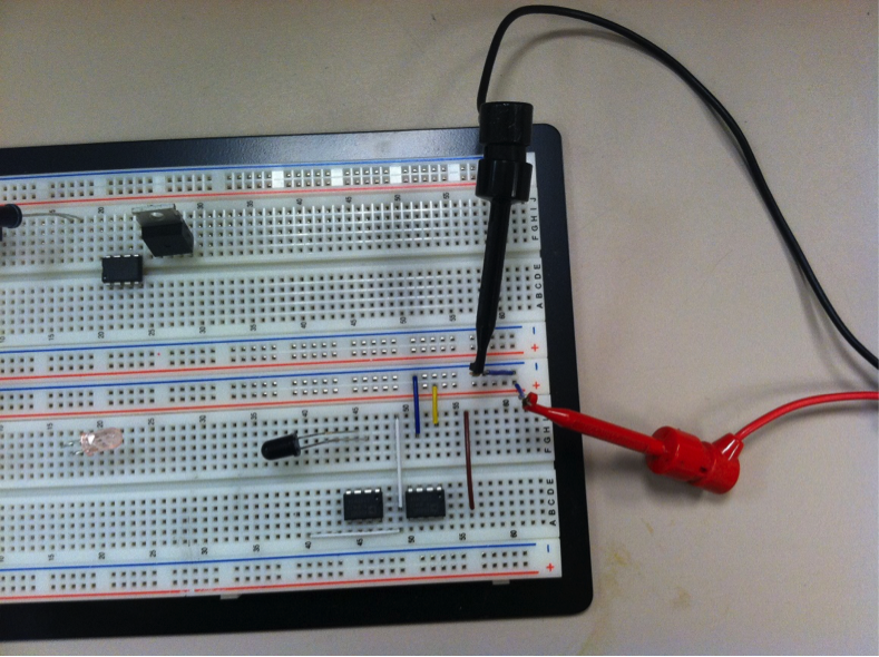
Figure 6
Figure 6 shows how to route (+) and (-) of the power supply to your circuit. The blue wire, which is inserted into the breadboard, shows how to couple the (-) of the power supply to your circuit. The blue wire is inserted in the blue (-) row and the other end of the blue wire is inserted into your circuit. The yellow wire, which is inserted into the breadboard, shows how to couple the (+) of the power supply to your circuit in the same way as how the blue wire was described. Using this method of power supply distribution will keep your breadboard neat, making it easier to analyze and troubleshoot. Also note how flat the inserted wires lay on the breadboard. You are encouraged to make your wire connections in the same way, which will again make analyzing and troubleshooting easier.
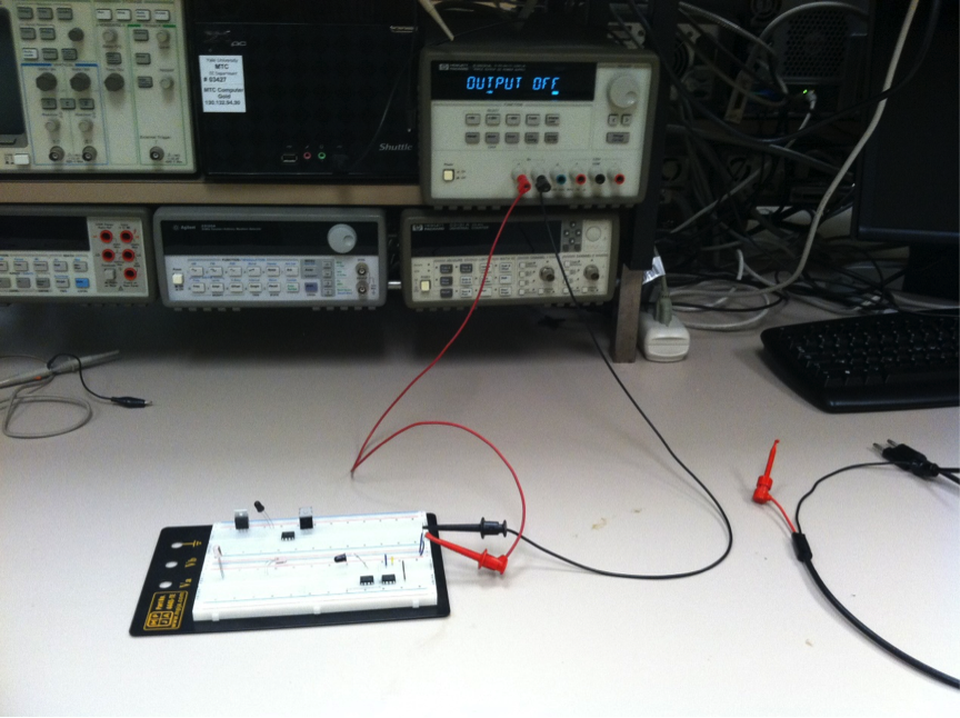
Figure 7
Figure 7 shows an alternative way of coupling a power supply to a breadboard, using cable, which have banana plugs inserted into the power supply, and cue ball clips, which are clipped to wires inserted into the breadboard’s blue (-) and red (+) rows.
Once the power supply is coupled to your circuit on the breadboard, you must turn on the power supply and supply power to your circuit.
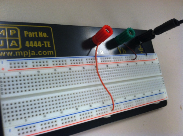
Figure 8
Some breadboards come with receptacles that allow you to plug power supply banana plugs directly into the breadboard. Figure 8 shows the black, or power supply ground lead plugged into a breadboard receptacle. Please note that you will have to connect a wire from the receptacle to the appropriate breadboard power row. Also shown in Figure 8 are the red and green receptacles wired to the breadboard. The red and green receptacles may be coupled to the power supply to supply two separate power supplies to the breadboard. Note that the wires coming from the red and green receptacle are inserted into two different red (+) rows of the breadboard. These two red (+) rows are not shared and can serve as two distinct “sources” for your circuit.
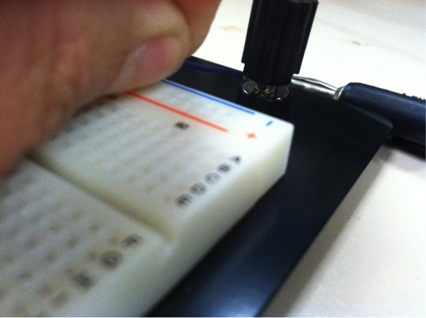
Figure 9
In Figure 9, connect the receptacle by unscrewing the receptacle and inserting a wire into the exposed hole, then tighten down the receptacle. Please be careful to not insert wire insulation into the receptacle’s hole because that will isolate the power supply from your circuit. Only insert bare wire into the hole. Then insert the other end of the wire into the appropriate breadboard power row.
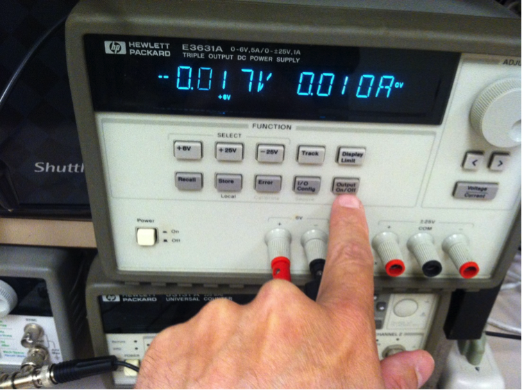
Figure 10
Turn the power supply on by pressing the power button in the lower left corner of the power supply’s front panel. When the power supply initially powered on, the outputs of the power supply will be turned off. Turn the power supply’s outputs on by pressing the “Output On/Off” button as shown in Figure 10.
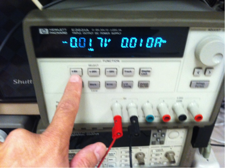
Figure 11
Next, select the power supply you want to use. In Figure 11, the +6 VDC power supply is being selected. This enables the +6V power supply, which will then supply power to the +6V output terminals.
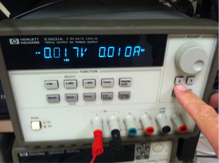
Figure 12
Figure 12 shows using the arrow keys on the power supply to move the significant digit. This power supply is capable of 1mV adjustment.
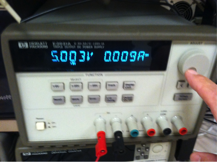
Figure 13
Figure 13 shows using the round knob to change the output level of the power supply.
At this point, you should be able to navigate the layout of a breadboard to build a circuit and couple a power supply to your circuit. The remaining parts of this presentation will cover input stimulus and output measurement. Input stimulus to your circuit may be Direct Current (DC), where a power supply would be used (power supplies serve double duty as supplying power to your circuit and supply input stimulus) and Alternating Current (AC), where a function generator would be used.
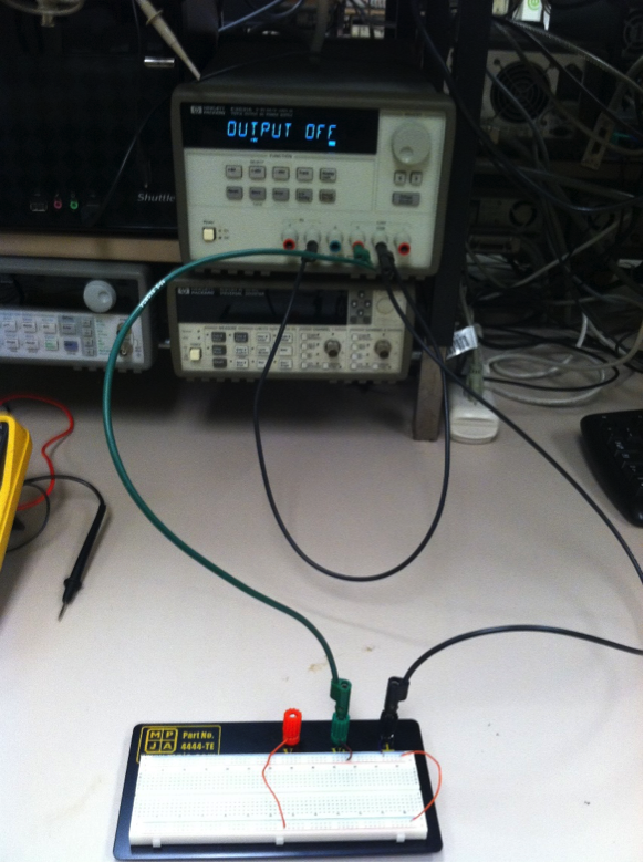
Figure 13a
Figure 13a shows how to setup two power supplies to a breadboard. The most important thing about setting up two power supplies for a circuit is that grounds of both power supplies must be coupled together, as shown in Figure 13a. Note the black cable shorting the grounds of the +6V and the +25V power supplies together, and the junction of the shorted grounds is coupled to the breadboard. This ensures that both power supplies explicitly share the same ground. Do not short the power side of the power supplies to each other or to ground.
Input Stimulus
Using a power supply as an input stimulus is accomplished in the same way as it’s used to supply circuit power. It should be noted that all three power supplies within the power supply case may be used independently. You may have use of the +6v, +25v, and -25v supplies as separate isolated supplies. Just hook it up and select the power supply you want to adjust. Selecting another power supply will NOT turn off any other power supplies, which will remain powered on if you powered them on.
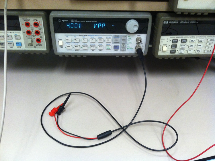
Figure 14
Figure 14 shows the function generator. You couple the function generator to a breadboard with a cable that has a Bayonet Neill-Concelman (BNC) connector, which couples to the function generator, and cue ball clips, which clop to inserted wires in a breadboard as in Figure 15.
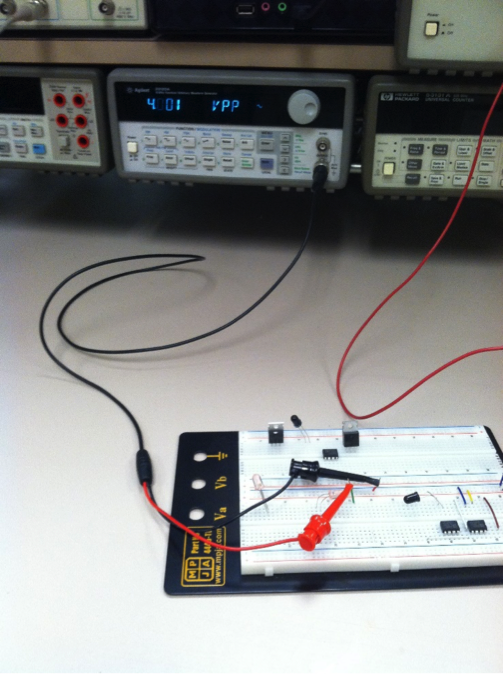
Figure 15
In Figure 15, note that the black (ground) cue ball is clipped to a breadboard wire, which is inserted in the blue (-) row, which is also connected to the power supply ground, or (-). By doing this, you “reference” the ground of the function generator to the ground of the power supply. This is important because all instruments must be grounded, or referenced together. If this is not done, a ground loop will form, which is current flowing between the grounds of instruments, which will cause offset voltages and can make measurement results inaccurate. This can also cause problems within your circuit.
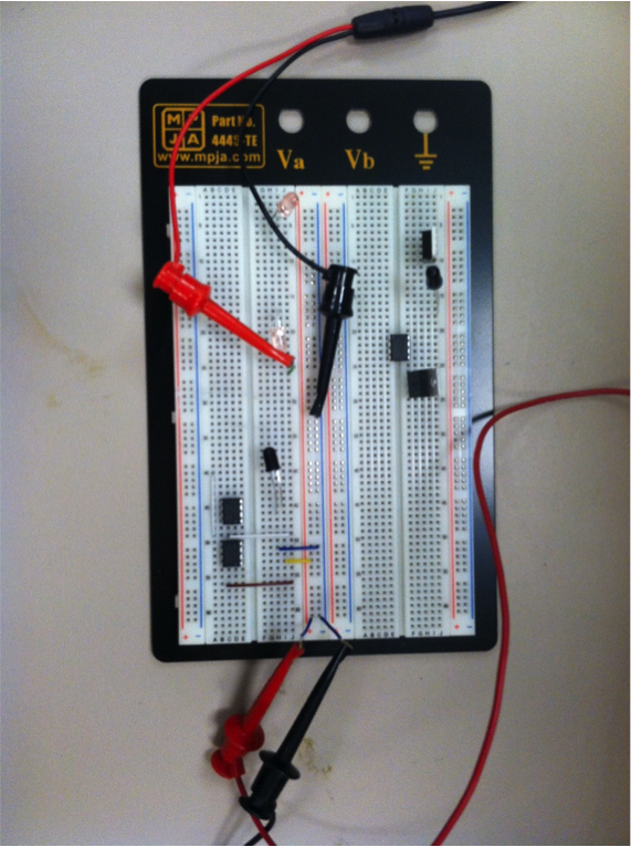
Figure 16
Figure 16 shows the function generator coupled to the breadboard on the top and the power supply coupled to the breadboard on the bottom. Again, note that the grounds are connected together via the blue (-) row of the breadboard. The red cue ball coming from the function generator is couple to a wire that is embedded in the one of the horizontal rows of the breadboard, which is supplying AC waveforms to the horizontal row between the breadboard’s red line (where the power supply is connected) and the center trough. The waveform of the function generator is available on all pins within the horizontal row, located between the breadboard’s red line and center trough.
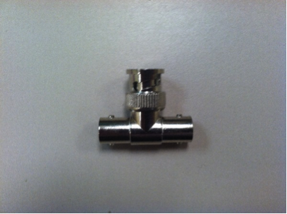
Figure 17
A BNC “T” may be used to split the output of the function generator. Splitting the output of the function generator allows you to apply one side of the BNC “T” to your circuit, and apply the other side to one of the channels of the oscilloscope. This will allow you to monitor and compare internal and output circuit waveforms to the input waveform, which allows you to make relative waveform measurements between the input of the function generator and the various parts of your circuit.
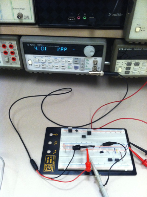
Figure 18
Figure 18 shows the BNC “T” coupled to the function generator, and the BNC/cue ball cable coupling the function generator to the breadboard. Note the other side of the BNC “T” is available to couple another BNC cable, which will be coupled to the oscilloscope.
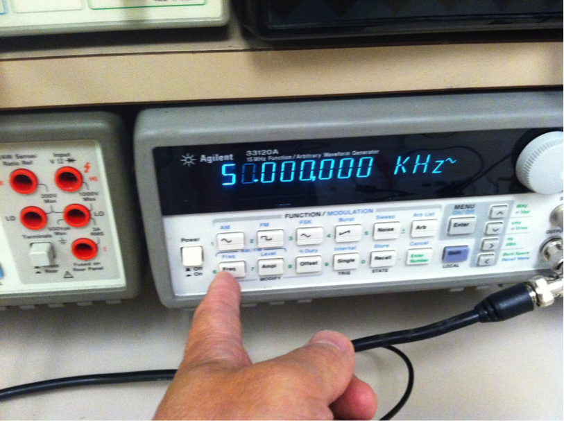
Figure 19
Pressing the “Freq” button on the function generator will allow you to change the frequency output of the function generator, as seen in Figure 19. The arrow keys on the right side of the function generator’s front panel function the same way as the power supply, allowing you to select the digit you want to change, as in Figure 20. The round knob also functions in the same manner as the round knob on the power supply, which will change the selected digit to the needed value.
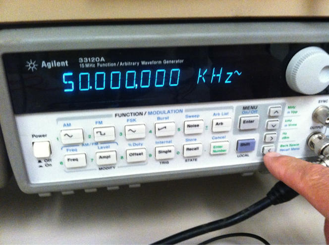
Figure 20
The “Ampl” button on the front panel of the function generator will allow you to change the amplitude of the waveform. The operation of changing the amplitude of the waveform is similar to changing the frequency.
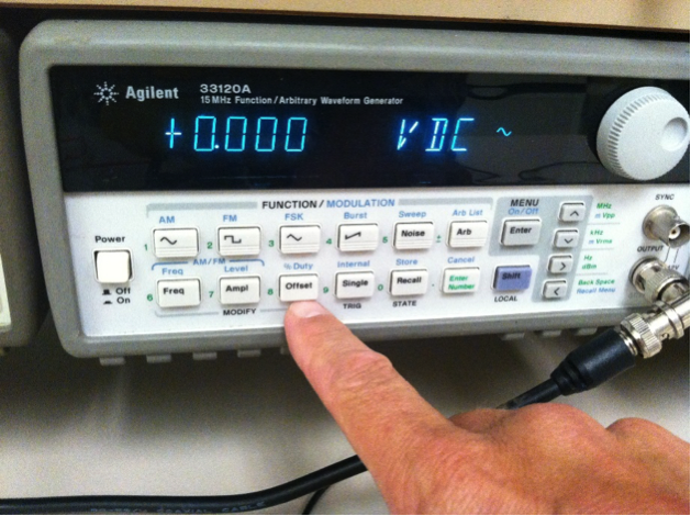
Figure 21
Figure 21 shows the “Offset” button. This function generator option will add a DC voltage level to the output waveform of the function generator. Without offset (0.0VDC), the waveform coming out of the function generator will swing about 0 VDC, which means if you select a 4.0 Vpp (Volts Peak-to-Peak), the output waveform will swing between +2.0v and -2.0v. If you select an offset of 2.0 VDC for the same 4.0 Vpp waveform, then the resulting waveform coming out of the function generator will swing about +2.0 VDC or between +4.0v and 0.0v. This is an important function generator feature and will help you understand how you are stimulating your circuit. The function generator has various waveform outputs, which are Sine Wave (Figure 22), Square Wave (Figure 23), Triangle Wave (Figure 24), and Ramp (also known as Sawtooth)(Figure 25).
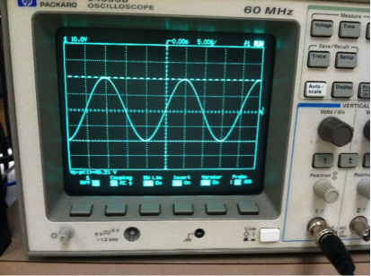
Figure 22
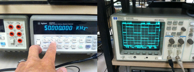
Figure 23
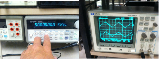
Figure 24
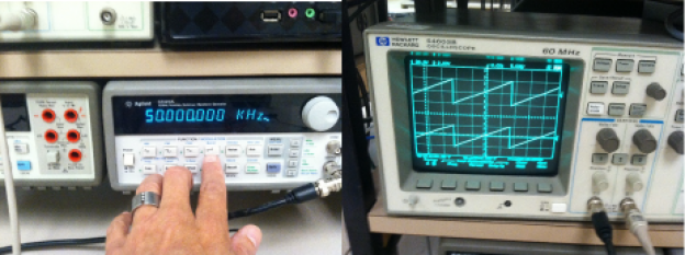
Figure 25
Note that Figures 23-25, there are two waveforms, because a BNC “T” is coupled to the function generator, and the oscilloscope is monitoring both the output waveform of the function generator, which is the input waveform to the circuit, and another point within the circuit. This allows for a relative comparison between the input waveform and waveforms within the circuit.
We have now covered supplying power to your circuit and we have covered input stimulus of your circuit. The remaining part of this presentation will cover output measurement of your circuit, which we will employ the use of an oscilloscope and digital volt/ohm meter.
Output Measurement
The oscilloscope is used to graphically capture, evaluate, and compare AC waveforms and DC levels. The digital Volt/ohm meter, or Digital Multimeter (DMM) is used to measure non-graphic AC and DC voltage and current levels, and measure resistance. The oscilloscope allows us to see how parts of electronics systems work like we would visually see how mechanical systems work. The oscilloscope is a time domain instrument, which means that it shows us changes in voltage level over time. This means we can get timing information on waveforms and the inverse of time, which is frequency. We can measure time, frequency, volts peak-to-peak (Vpp), minima and maxima of the waveform, and root-mean-square (rms) of waveforms. All of this is important in verifying our circuits.
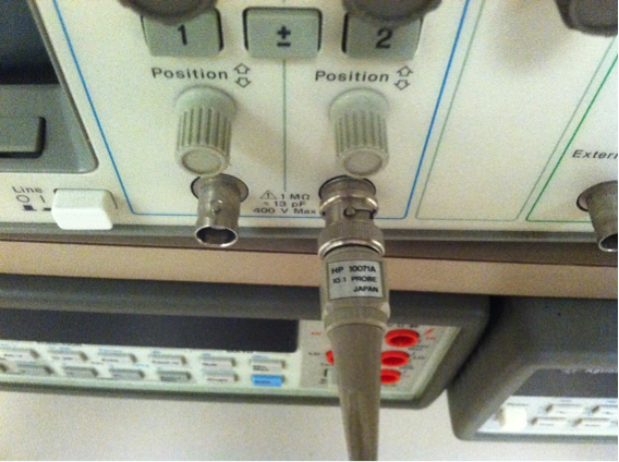
Figure 26
Figure 26 shows the inputs to the oscilloscope (scope). The oscilloscopes in these labs have two inputs called channels. Scopes typically can have up to four channels. Probes attach to oscilloscopes as illustrated in Figure 26, via BNC connectors. It is important to read the label on scope probes. The scope probes that you will be using in this lab are 10:1, which means these probes have an attenuation of 10. There are also scope probes that are 1:1, which means no attenuation. The reason for attenuation is because a scope can capture waveforms of up to 400 Vpp. Using an attenuated probe makes it easier to see small waveforms.
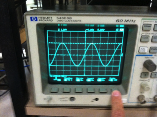
Figure 27
You must tell the scope what kind of probe you are using, whether it is 1:1 or 10:1. You do this by pressing the “1” button found just to the right of where the finger is pointing in Figure 27, between the gray knob and the white knob, then pressing the button where the finger is pointing until the scope reads the same as the scope probe label. If you notice that your function generator is putting out a 4.0 Vpp and the peak-to-peak value on your scope is reading 40 Vpp, you will want to adjust the scope from thinking you have a 1:1 probe to having a 10:1 probe.
Scopes have a nice feature built-in, which is called “Auto-scale.” The Auto-scale button is a white button, and it is located just to the right and just above the middle of the screen in Figure 28. Auto-scale will capture most waveforms. For waveforms that are difficult to capture, please refer to the oscilloscope’s documentation on “triggering.”
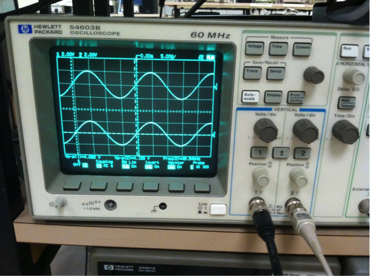
Figure 28
Figure 28 shows both channels being used. Channel 1, which is on the left, is receiving the output waveform of the function generator (input waveform to the circuit), and channel two, which is on the right, is monitoring the circuit.
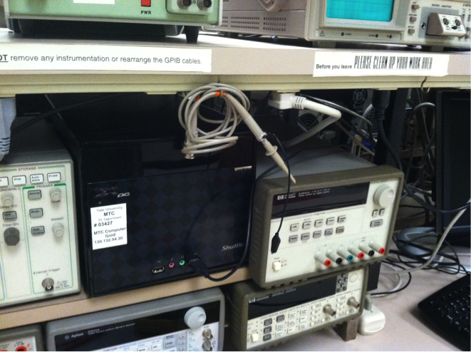
Figure 29
Scope probes hang from the bench as illustrated in Figure 29. Please return them to the same place when you are done using them.
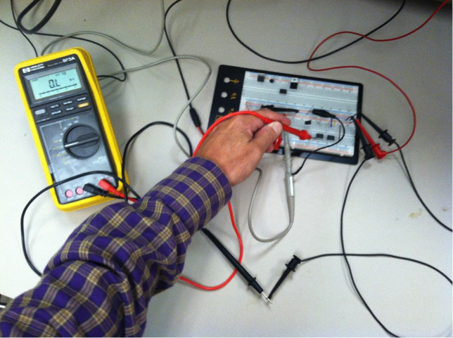
Figure 29a
Figure 29a shows the use of the DMM, which is the meter with the yellow plastic case. The DMM comes equipped with probes, which are used to probe various parts of electronic circuits, to measure voltage. Do not try to measure resistance to a circuit that has voltage applied, because your measurement will be false. The DMM puts out a known voltage and measuring resulting current to calculate resistance. If you try to measure resistance on a component in a powered circuit, you will not have a valid reading because to the voltage being applied from the power supply. In Figure 29, you can see that the negative (black) probe is coupled to the blue (-) breadboard row, which also has the negative terminals of the power supply and function generator coupled to it. All grounds must be the same as the circuit’s ground. The black DMM probe is coupled to the breadboard using a cable having cue ball clips on both ends. The color on the cable should be kept consistent with whether you are coupling power/signal (red), or ground (black). If you cannot find the appropriate colored cable, make use of another color, but keep track of the color difference, which can become confusing. You may also connect the positive DMM probe using the same type of cable, freeing your hands to operate other equipment.
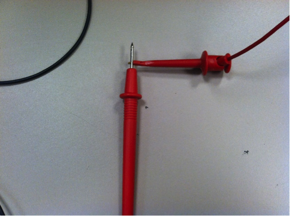
Figure 30
Figure 30 shows a cue ball clip connecting to a DMM probe.
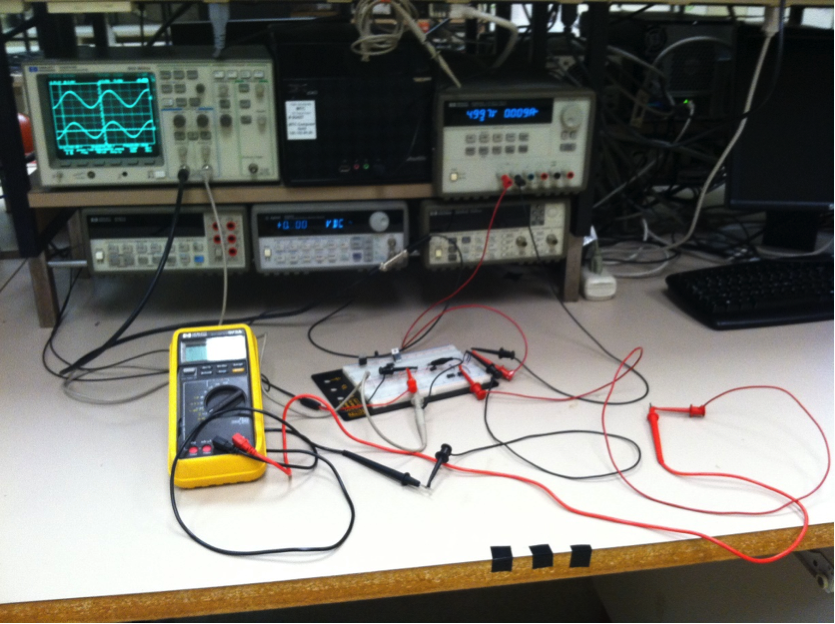
Figure 31
Figure 31 shows a typical circuit setup, using a breadboard, power supply, function generator, oscilloscope, and DMM.
Further Resources
This guide has only covered the basics. For detailed instructions on the operation of all equipment found in room C048 please refer to:
http://mtc.yale.edu/room-c048